Emit #6 – AirSensEUR Calibration

This is Emit #6, in a series of blog-posts around the Smart Emission Platform , an Open Source software component framework that facilitates the acquisition, processing and (OGC web-API) unlocking of spatiotemporal sensor-data, mainly for Air Quality and other environmental sensor-data like noise.

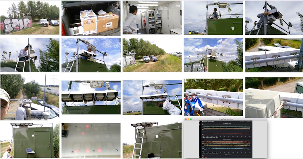
In Emit #5 – Assembling and Deploying 5 AirSensEURs… , I described how , with the great help of Jan Vonk from RIVM, we placed five AirSensEUR (ASE) air quality stations at the RIVM reference site near the A2 Highway at Breukelen. For about 2.5 months raw data was gathered there while the RIVM station was gathering its data to be used as reference for calibration.

Now “calibration” is a huge and increasingly important topic when using inexpensive sensors for measuring Air Quality. Within the Smart Emission project we have been applying Artificial Neural Networks to calibrate the gas-sensors within the Josene stations. See also the SE documentation . These sensors were so called metaloxide (MICS) sensors from SGX Sensortech Limited .

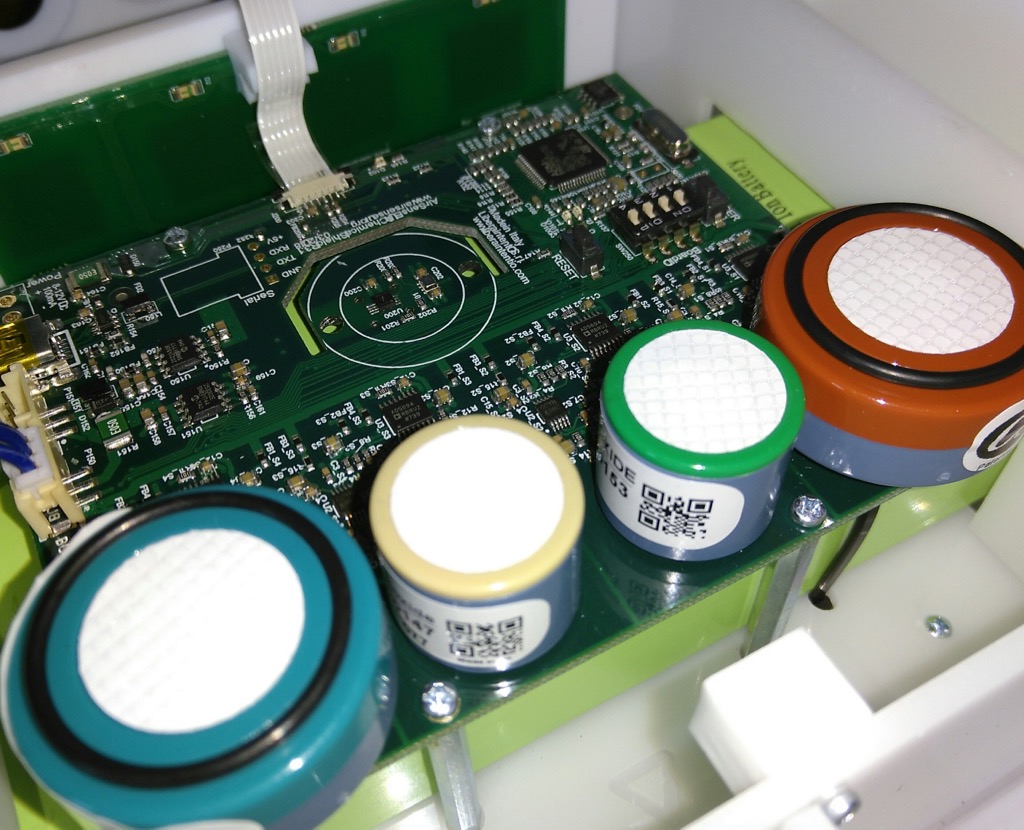
The AirSensEURs contain electrochemical sensors from AlphaSense . Several sources like RIVM , state that these sensors are more accurate (than metaloxide sensors), but at the same time need per-sensor calibration.

Within the ASE boxes the following four gas-sensors were applied:

• NO2 (Nitrogen Dioxide): the NO2-B43F , see datasheet .
• NO (Nitric Oxide): the NO-B4 , see datasheet .
• O3 (Ozone): the OX_A431 , see datasheet .
• CO (Carbon Monoxide): the CO-A4 , see datasheet .

The calibration to be applied is based on Regression Analysis . This and other calibration-methods have been investigated and evaluated for many types/brands of sensors by the EC-JRC team. Read all in this landmark article and other references there.

The complete timeline was as follows. Each phase will be expanded below.

1. Aug 1, 2018 – Okt 9, 2018
   Raw ASE and RIVM reference data collection (Breukelen site)

2. Okt 10, 2018 – Nov 2, 2018
   All ASEs deployed at their target locations

3. Nov/dec 2018
   Calibration performed by Michel Gerboles at the EC-JRC lab

4. Jan 2019
   Calibration formulas implemented in Smart Emission (SE) platform

5. Feb 2019
   All ASE calibrated gas-data continuously available via SE viewers/APIs

6. Feb 2019
   Analysis of the calibration (SE Python Stetl ) implementation results

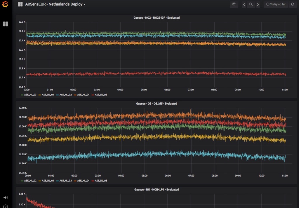
ad 1) The five ASE Boxes were mounted on a horizontal pole and connected to WIFI and current. As end-result all boxes were publishing their raw data to the SE InfluxDB Data Collector and were visible in the SE Grafana raw data viewer .

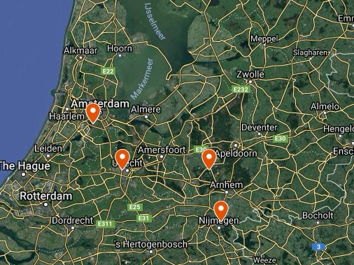
ad 2) The picture below shows ASE_NL_01 (left above) through _05 clockwise at their deployment sites. ASE_03 and 04 (right below) were at a single location.

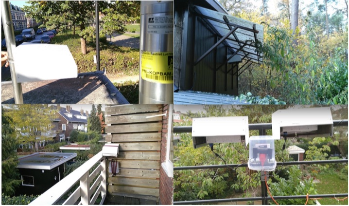
ASE_NL 01 was deployed at an RIVM site in Nijmegen. This allowed us to verify its calibration with different reference data as with which it was calibrated! See below.

ad 3) The calibration was performed by EC-JRC (M. Gerboles) using R and ShinyR webapp. All sources can be found in this EC-JRC GitHub repo . This process is quite intricate and a bit hard to explain in the context of a blog-post paragraph. I’ll try a summary:

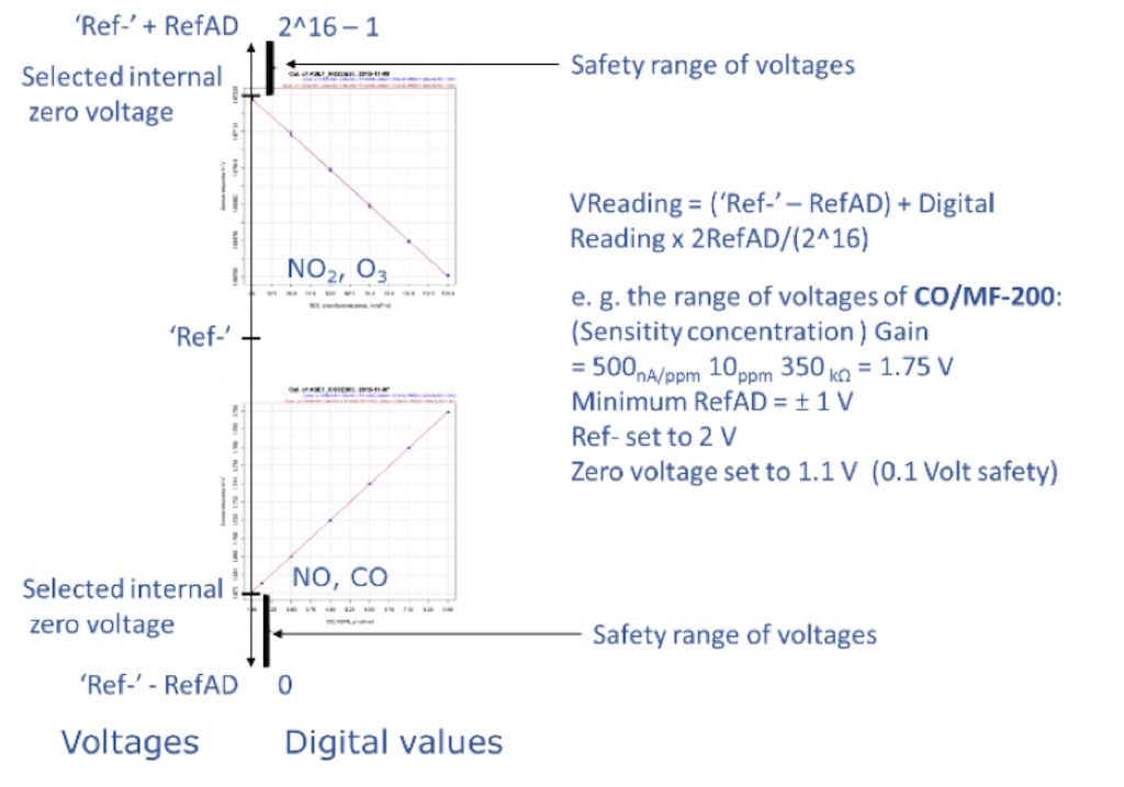
Sensor values are digital readings (0..65535). This is effected by the electrical circuitry within each ASE, for optimal gain. To calculate back to mV and nA a per-sensor (brand+type) calculation is required first before applying any regression formula. A bit is explained in the image below.

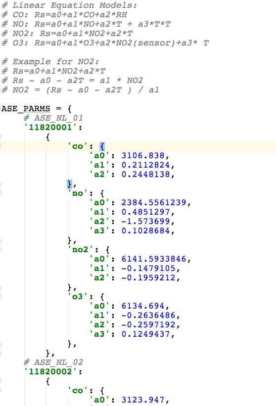
The second outcome is a per-individual-sensor regression formula. This is for most sensors a linear equation. For O3 (OX_A431) the formula is polynomial, as O3 readings are influenced by NO2 concentration. Below is an example as later implemented in Python using SE Stetl ETL

The main three outcomes of the calibration are:

• the parameters for digital to nA calculation (per sensor brand+type)
• the linear (polynomial) equations for nA to concentration (ug/m3)
• the per-individual-sensor parameters (a0-a3)

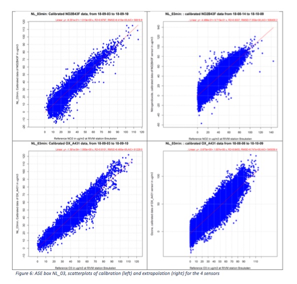
Above some scatterplots made for ASE Box 3 NO2 and O3.

ad 4) Knowing all equations and their parameters from step 3 above, I attempted to integrate this in the continuous ETL within the Smart Emission Platform. Up to now the platform supported only a single sensor station type: the Intemo Jose(ne). As the platform is fed by harvesting raw data from a set of remote APIs provided by Data Collectors, it was relatively easy to add sensor(-station)-metadata and extend the Refiner ETL to apply calibration algorithms driven by that metadata.

So for Josene stations the existing ANN calibration would still be applied, while for ASE stations per-sensor linear equations would be performed. All parameterization was already configurable using the Device, DeviceDefs, DeviceFuncs abstractions in the SE Stetl implementation . Recently, to allow stations that already send calibrated values, I introduced the Vanilla Device starting with harvesting Luftdaten.info stations (more in a later post).

The formula’s as applied in Python SE Stetl are as follows:

1STEP 1a - Digital to Voltage (V)
2V = (Ref - RefAD) + (Digital+1) /2^16 x 2 x RefAD

1STEP 1b - Voltage (V) to Ampere (I) as Ri
2I = 10^9 V/(Gain x Rload)

1STEP 2 - Ampere (I) to concentration (ug/m3) - Example
2I=a0+a1*NO2+a2*T

1==> NO2 = (I - a0 - a2 * T) / a1
2a0-a2 has specific values for each NO2-B43F sensor.

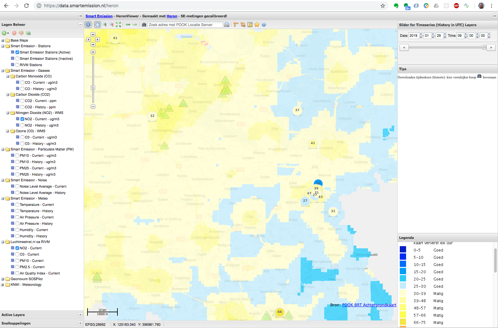
Now that these formulas and their parameters were implemented, near-realtime values could be made visible in all SE apps (viewers) and APIs such as the SmartApp and the Heron Viewer .

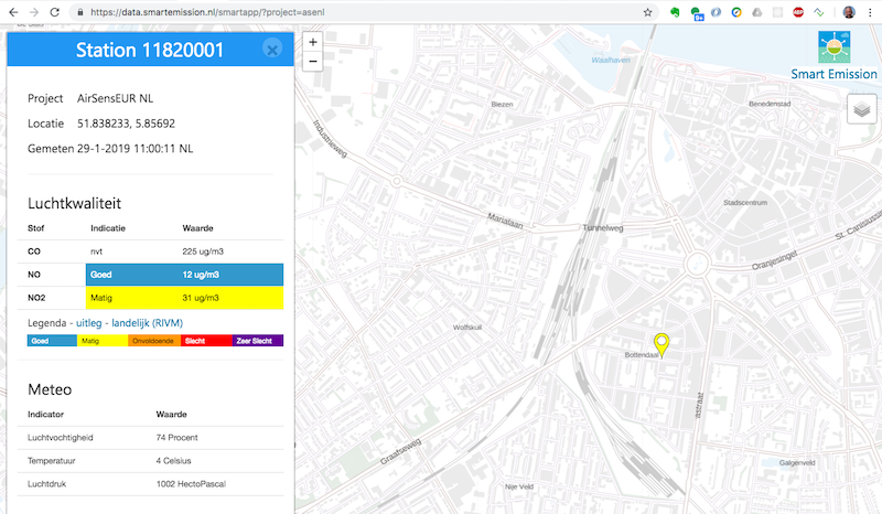
Within the Heron Viewer we can compare for example NO2, not only with Josene measurements, but also with official RIVM values.

Also the data is available through all SE OGC APIs , for example the SensorThings API .

ad 6) The moment of truth! How well does the SE-based SE Stetl Python calibration results fit with the original RIVM values? One of the advantages of Data Harvesting (opposed to data push) is that we can switch back in time, i.e. restart harvesting from a given date. Harvesting and continuous calibration was restarted from august 1, 2018, the start of the calibration period at the RIVM station. Using a Grafana panel that displays both RIVM and SE-calculated values we can graphically see how well the data aligns.

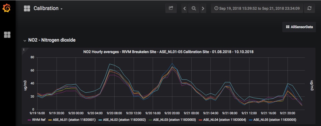
What we can see from the above image, is that visually the data aligns very well, here for NO2. The purple graph is the official RIVM measurement. Only station ASE NL 02 is not completely aligned.

To also have some numeric proof and a more objective comparison, I dived in scatterplot and numerical analysis in Python. Apart from scatterplots that show calculated (Y) agains RIVM ref values (X) I calculated the “R-squared” and “slope” for fitting indicator values. This was also my first serious use of Python libs like Scipy, Pandas, Seaborn and Numpy (you’re never too old to become a data-scientist!).

As all SE calibrated data is also stored in InfluxDB with RIVM refdata harvested from their SOS, it was easy to fetch values for the plots/calculations.

Objectivity could be effected since station ASE NL 01 was finally deployed (okt 2018) in Nijmegen, also next to an RIVM station. So the calibration calculations from RIVM refdata in Breukelen could be compared to “Nijmegen”. The implementation for making these scatterplots can be found here . Lets look at some results, mainly for NO2, as I consider this one of the most important AQ indicator gasses.

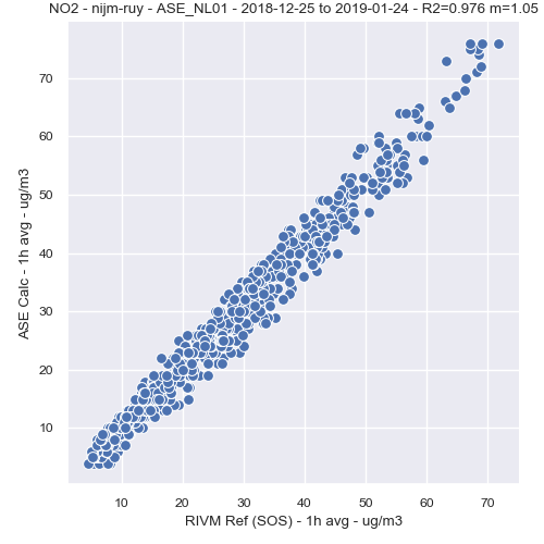
I like this image a lot as it shows an almost ideal alignment with an R2 of 0.976 and slope of almost 1. Mind: calibration was thus done at a very different site (about 80 km west) and AQ condition (highway) as the deployment (city street).

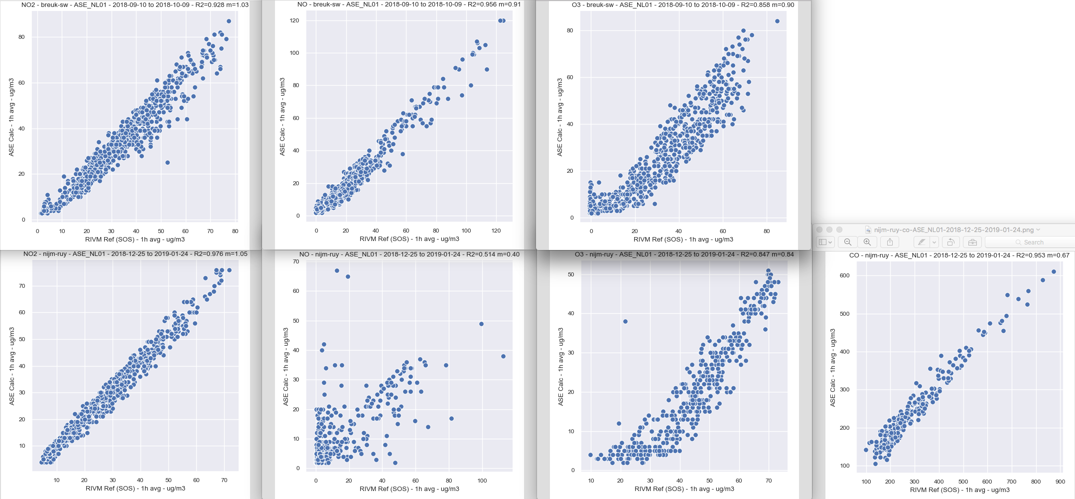
Above are plots for the other gasses as well. First row in Breukelen (no ref CO available in RIVM SOS), front row in Nijmegen. Only NO in Nijmegen is a bit problematic.

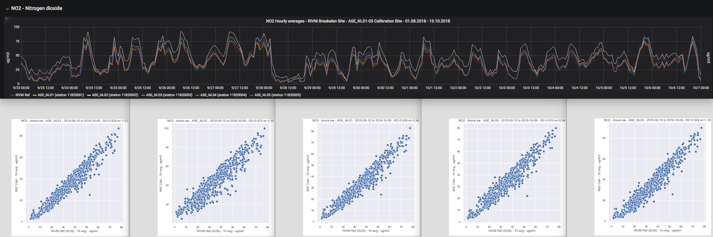
To close off: this last image above shows NO2 fit at the Breukelen station for all five ASE boxes. Also quite good.

What to conclude? First of all AirSensEUR is a major step forward in affordable accurate AQ sensing. We hope to expand the community.

AlphaSense NO2 electrochemical sensors appear quite accurate, but calibration requires quite some effort, plus calibration formulas apply per individual sensor. Would automatic per-sensor ANN be less time-consuming and still accurate? Something I would like to investigate.

The Smart Emission project and platform is still going strong, running within a Kubernetes Cloud maintained by Dutch Kadaster.

Next emit will discuss how I integrated data from the amazing Luftdaten.info project for the municipality of Nijmegen.